Part 1

Download Cook County Assessor’s Residential Modeling Characteristics (Chicago). Load this into R using read_csv. Either set your file directory using a R project or create a variable with the path of the folder the file is located in. Do not use absolute paths!

Note you can also use urls in read_csv directly.

library(tidyverse)
ccao <- read_csv('../../../files/Assessor__Archived_05-11-2022__-_Residential_Modeling_Characteristics__Chicago_.zip')

Part 2

How many single family homes are included in the data? Out of all the residential properties, what is the most common class? Hint: You may have to look up appropriate Property Classes.

#https://prodassets.cookcountyassessor.com/s3fs-public/form_documents/classcode.pdf
ccao %>% filter(`Property Class` %in% c(202, 203, 204, 205, 206, 207, 208, 209, 210, 234, 278)) %>%
  nrow()

## [1] 289388

ccao %>% count(`Property Class`) %>% slice_max(n, n=1) #299 is condos

## # A tibble: 1 x 2
##   `Property Class`      n
##              <dbl>  <int>
## 1              299 236813

Part 3

Using lubridate, calculate some information on sales:

• Number of sales in any January
• Number of sales in 2020
• Number of sales on January 2020
• Number of sales on your birthday (or favorite day)
• Number of sales on Wednesday (or your favorite day of the week)

library(lubridate)

ccao %>% select(`Sale Date`)

## # A tibble: 678,656 x 1
##    `Sale Date`
##    <chr>      
##  1 <NA>       
##  2 <NA>       
##  3 <NA>       
##  4 <NA>       
##  5 <NA>       
##  6 <NA>       
##  7 <NA>       
##  8 <NA>       
##  9 <NA>       
## 10 <NA>       
## # ... with 678,646 more rows

ccao <- ccao %>% mutate(sdate = mdy_hms(`Sale Date`))

ccao %>% filter(month(sdate) == 1) %>% nrow()

## [1] 6591

ccao %>% filter(year(sdate) == 2020) %>% nrow()

## [1] 24701

ccao %>% filter(floor_date(sdate, 'month') == ymd('2020-01-01')) %>% nrow()

## [1] 1813

ccao %>% filter(day(sdate) == 23 & month(sdate) == 6) %>% nrow()

## [1] 67

ccao %>% 
  filter(wday(sdate, label = TRUE) == 'Wed') %>% nrow()

## [1] 15540

Part 4

Using ggplot2, make the following plots:

1. Average sale price by number of bedrooms. Use class 203 only and only include values with at least 1000 sales.

library(scales)
graph_data <- ccao %>% filter(`Property Class` == 203) %>% 
  group_by(Bedrooms) %>%
  summarize(avg_sp = mean(`Sale Price`, na.rm=T),
            count = n()) %>%
  filter(count >= 1000)

ggplot(graph_data, aes(x=Bedrooms, y=avg_sp)) +
  geom_bar(stat='identity') +
  scale_y_continuous(labels=dollar) +
  theme_bw() +
  labs(y='Average Sale Price', title='Average Sale Price by Bedrooms')

2. Sales over time. First, show 2018 to present.

graph_data2 <- ccao %>% filter(!is.na(sdate)) %>%
  group_by(sdate = floor_date(sdate, 'week')) %>% 
  summarize(count = n())

ggplot(graph_data2, aes(x=sdate, y=count)) +
  geom_line(stat='identity') +
  theme_bw() +
  labs(x='Week', y='Number of Sales', title='Weekly Sales in Chicago')

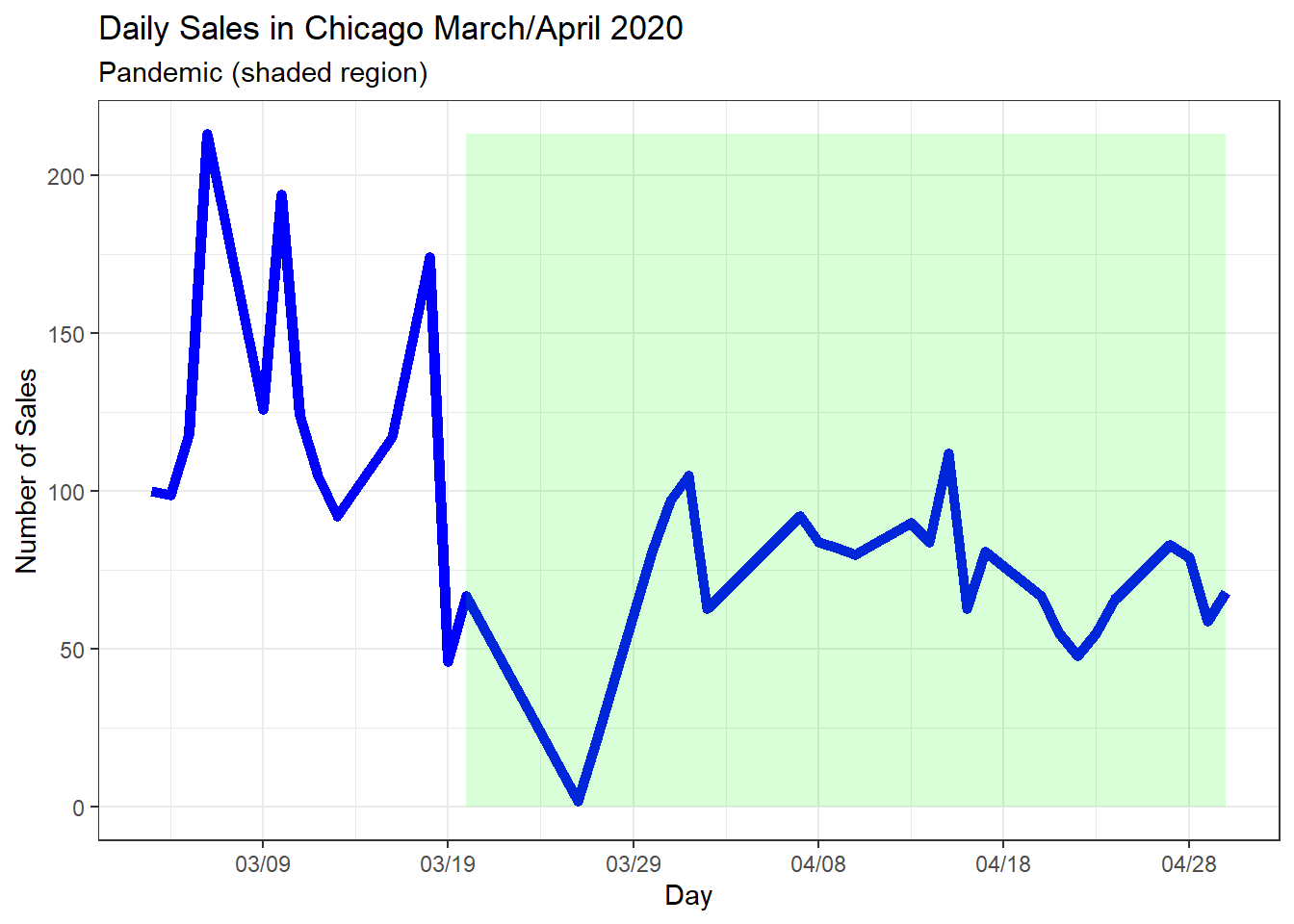
3. March and April 2020 sales. Then, use scale_x_date (or scale_x_datetime if appropriate) on the x-axis to set the date breaks 10 days apart and date labels as month/day of month (e.g. 3/9). Shade in the region of the graph after the pandemic began.

graph_data3 <- ccao %>% filter(!is.na(sdate)) %>%
  filter(between(ymd(sdate), ymd('2020-03-01'), ymd('2020-04-30'))) %>% #a more natural way to do this
  group_by(sdate = ymd(floor_date(sdate, 'day'))) %>% #using dates is easier instead of datetimes sometimes
  summarize(count = n())

ggplot(graph_data3, aes(x=sdate, y=count)) +
  geom_line(stat='identity', color='blue', size=2) +
  scale_x_date(date_breaks='10 days', date_labels = '%m/%d') +
  geom_rect(fill='green', alpha=0.005, aes(xmin=ymd('2020-03-20'), xmax=ymd('2020-04-30'), ymin=0, ymax=max(graph_data3$count))) +
  theme_bw() +
  labs(x='Day', y='Number of Sales', title='Daily Sales in Chicago March/April 2020', subtitle='Pandemic (shaded region)')