This assignment is ungraded. I encourage you to review the problems to see if (1) you know how to do them or (2) if you know how to google how to do it. If either path forward escapes you, I suggest that you complete this assignment.
Part 1
Exercise 7.2.3 from Data Science for Public Policy. Data can be found here.
- Graph and regress sale price against gross square feet interpret the results
sale_df <- read_csv("https://raw.githubusercontent.com/DataScienceForPublicPolicy/diys/main/data/home_sales_nyc.csv")

ggplot(data = sale_df, aes(x = gross.square.feet, y = sale.price)) +
  geom_point(alpha = 0.15,
             size = 1.2,
             colour = "blue") +
  scale_x_continuous("Property size (gross square feet)", labels = scales::comma) +
scale_y_continuous("Sale price (USD)", labels = scales::comma) 
reg_est <- lm(sale.price ~ gross.square.feet, data = sale_df)

summary(reg_est)
##
## Call:
## lm(formula = sale.price ~ gross.square.feet, data = sale_df)
##
## Residuals:
## Min 1Q Median 3Q Max
## -1700116 -212264 -44958 138638 8661923
##
## Coefficients:
## Estimate Std. Error t value Pr(>|t|)
## (Intercept) -42584.389 11534.260 -3.692 0.000223 ***
## gross.square.feet 466.176 7.097 65.684 < 2e-16 ***
## ---
## Signif. codes: 0 '***' 0.001 '**' 0.01 '*' 0.05 '.' 0.1 ' ' 1
##
## Residual standard error: 463900 on 12666 degrees of freedom
## Multiple R-squared: 0.2541, Adjusted R-squared: 0.254
## F-statistic: 4314 on 1 and 12666 DF, p-value: < 2.2e-16Part 2
Reproduce this figure from tidymodels 3.3
 with the data from Part 1 replacing mpg with sale price for numeric variables.
corr_res <- map(sale_df %>%
                  select(where(is.numeric), -c(sale.price, borough, zip.code)),
                cor.test,
                y=sale_df$sale.price)
corr_res %>%
  map_dfr(broom::tidy, .id = "predictor") %>%
  ggplot(aes(x = fct_reorder(predictor, estimate))) +
  geom_point(aes(y = estimate)) +
  geom_errorbar(aes(ymin = conf.low, ymax = conf.high), width = .1) +
  labs(x = NULL, y = "Correlation with sale price") +
  theme_bw() +
  coord_flip()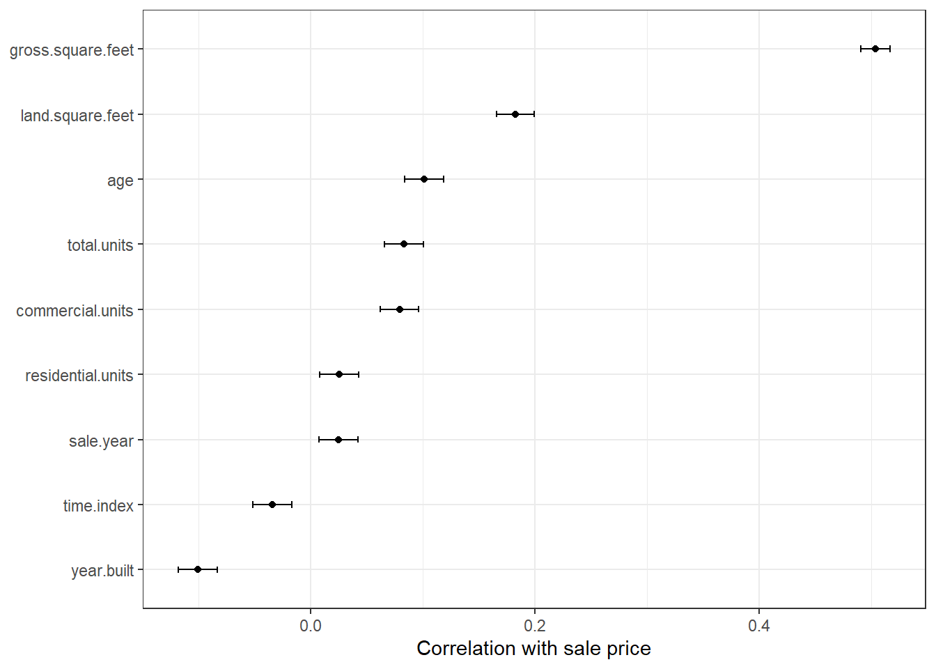
Part 3
Exercise 7.4.5
Estimate a set of regressions, evaluate the pros and cons of each, and select the “best” specification.
Create and analyze the following four models from the textbook and one of your own:
- Model 1 (mod1) regresses sales prices and building area
- Model 2 (mod2) adds borough as a categorical variable
- Model 3 (mod3) incorporates an interaction to estimate borough-specific slopes for building area
- Model 4 (mod4) adds land area
library(gridExtra)
# Simple regression
mod1 <- lm(sale.price ~ gross.square.feet,
           data = sale_df)
# With borough
mod2 <- lm(sale.price ~ gross.square.feet + factor(borough),
           data = sale_df)
# Interaction
mod3 <- lm(sale.price ~ gross.square.feet * factor(borough),
           data = sale_df)
# With Additional variables
mod4 <-
  lm(sale.price ~ gross.square.feet * factor(borough) + land.square.feet + age,
     data = sale_df)

sale_df <- sale_df %>% mutate(quarter = lubridate::floor_date(sale.date, 'quarter'))

mod5 <- lm(sale.price ~ gross.square.feet * factor(borough) + land.square.feet + age + factor(quarter),
     data = sale_df)

#Base
base1 <-
  ggplot(sale_df, aes(x = gross.square.feet, y = sale.price / 1000000)) +
  geom_point(colour = rgb(0, 0, 0, 0.1), size = 0.8) +
  geom_point(
    aes(x = sale_df$gross.square.feet, y = predict(mod1) / 1000000),
    colour = rgb(1, 0, 0, 0.2),
    size = 0.6
  ) +
  xlab("Gross Square Feet") + ylab("Sales Price ($MM)") +
  ggtitle(paste0("Model 1 (BIC = ", round(BIC(mod1)), ")")) +
  xlim(0, 3000) + ylim(0, 3)

#Base2
base2 <-
  ggplot(sale_df, aes(x = gross.square.feet, y = sale.price / 1000000)) +
  geom_point(colour = rgb(0, 0, 0, 0.1), size = 0.8) +
  geom_point(
    aes(x = sale_df$gross.square.feet, y = predict(mod2) / 1000000),
    colour = rgb(1, 0, 0, 0.2),
    size = 0.6
  ) +
  xlab("Gross Square Feet") + ylab("Sales Price ($MM)") +
  ggtitle(paste0("Model 2 (BIC = ", round(BIC(mod2)), ")")) +
  xlim(0, 3000) + ylim(0, 3)

#Base3
base3 <-
  ggplot(sale_df, aes(x = gross.square.feet, y = sale.price / 1000000)) +
  geom_point(colour = rgb(0, 0, 0, 0.1), size = 0.8) +
  geom_point(
    aes(x = sale_df$gross.square.feet, y = predict(mod3) / 1000000),
    colour = rgb(1, 0, 0, 0.2),
    size = 0.6
  ) +
  xlab("Gross Square Feet") + ylab("Sales Price ($MM)") +
  ggtitle(paste0("Model 3 (BIC = ", round(BIC(mod3)), ")")) +
  xlim(0, 3000) + ylim(0, 3)

#Base4
base4 <-
  ggplot(sale_df, aes(x = gross.square.feet, y = sale.price / 1000000)) +
  geom_point(colour = rgb(0, 0, 0, 0.1), size = 0.8) +
  geom_point(
    aes(x = sale_df$gross.square.feet, y = predict(mod4) / 1000000),
    colour = rgb(1, 0, 0, 0.2),
    size = 0.6
  ) +
  xlab("Gross Square Feet") + ylab("Sales Price ($MM)") +
  ggtitle(paste0("Model 4 (BIC = ", round(BIC(mod4)), ")")) +
  xlim(0, 3000) + ylim(0, 3)

grid.arrange(base1, base2, base3, base4, ncol = 2)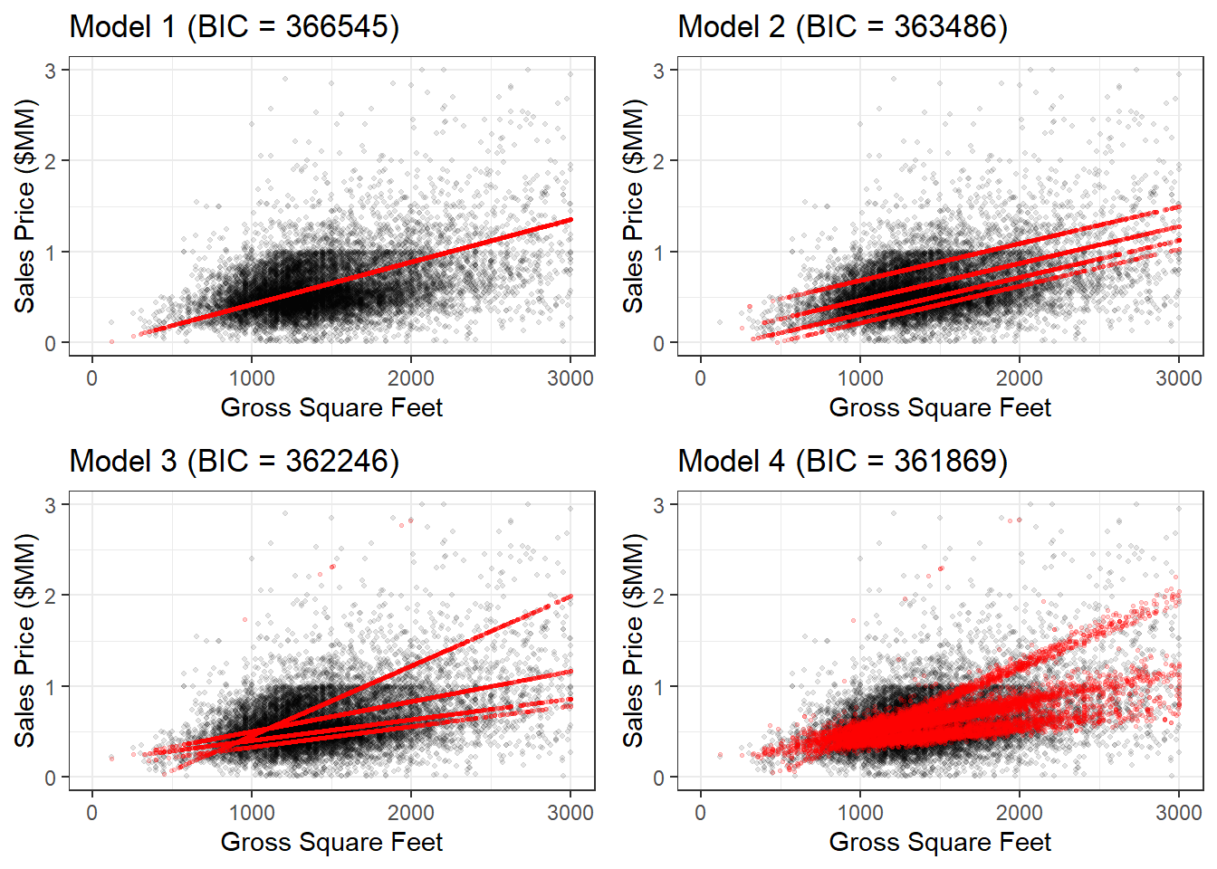
broom::glance(mod5)## # A tibble: 1 × 12
## r.squared adj.r.s…¹ sigma stati…² p.value df logLik AIC BIC devia…³
## <dbl> <dbl> <dbl> <dbl> <dbl> <dbl> <dbl> <dbl> <dbl> <dbl>
## 1 0.489 0.489 3.84e5 808. 0 15 -1.81e5 3.62e5 3.62e5 1.87e15
## # … with 2 more variables: df.residual <int>, nobs <int>, and abbreviated
## # variable names ¹adj.r.squared, ²statistic, ³deviancebroom::tidy(mod5)## # A tibble: 16 × 5
## term estimate std.error statistic p.value
## <chr> <dbl> <dbl> <dbl> <dbl>
## 1 (Intercept) 794057. 192345. 4.13 3.68e- 5
## 2 gross.square.feet 1032. 56.4 18.3 9.11e-74
## 3 factor(borough)2 -652250. 194929. -3.35 8.22e- 4
## 4 factor(borough)3 -1098488. 192639. -5.70 1.21e- 8
## 5 factor(borough)4 -611850. 192018. -3.19 1.44e- 3
## 6 factor(borough)5 -596887. 192362. -3.10 1.92e- 3
## 7 land.square.feet 37.3 1.86 20.1 3.31e-88
## 8 age -721. 154. -4.69 2.71e- 6
## 9 factor(quarter)2017-10-01 431. 13121. 0.0329 9.74e- 1
## 10 factor(quarter)2018-01-01 3506. 13441. 0.261 7.94e- 1
## 11 factor(quarter)2018-04-01 8800. 13278. 0.663 5.07e- 1
## 12 factor(quarter)2018-07-01 52101. 14444. 3.61 3.11e- 4
## 13 gross.square.feet:factor(borough)2 -866. 60.4 -14.3 3.18e-46
## 14 gross.square.feet:factor(borough)3 -291. 57.8 -5.04 4.76e- 7
## 15 gross.square.feet:factor(borough)4 -761. 57.4 -13.3 7.37e-40
## 16 gross.square.feet:factor(borough)5 -890. 57.6 -15.4 2.58e-53Part 4
In the class divvy example (see the lectures page for code/files), we had a lot of missing values in our data. We also didn’t have a very rigorous treatment of time/seasonality. Explore how impactful these issues are by creating a few different models and comparing the predictions using the workflows we saw from class in rsample (splitting data), parsnip (linear_reg, set_engine, set_mode, fit), yardstick (mape, rmse), and broom (augment).
divvy_data <- read_csv('https://github.com/erhla/pa470spring2023/raw/main/static/lectures/week_3_data.csv')

# split data

grouped <- rsample::initial_split(divvy_data)
train <- training(grouped)
test  <- testing(grouped)

# create parsnip model

lm_model <-
  parsnip::linear_reg() %>%
  set_engine("lm") %>%
  set_mode('regression') %>%
  fit(rides ~ solar_rad + factor(hour(started_hour)) +
           factor(wday(started_hour)) +
           factor(month(started_hour)) +
           temp + wind + interval_rain + avg_speed, data=train)

# predict and augment

preds <-
  predict(lm_model, test %>% filter(month(started_hour) >= 5))

test_preds <- lm_model %>%
  augment(test %>% filter(month(started_hour) >=5))

# evaluate

yardstick::mape(test_preds,
     truth = rides,
     estimate = .pred)
## # A tibble: 1 × 3
## .metric .estimator .estimate
## <chr> <chr> <dbl>
## 1 mape standard 121.yardstick::rmse(test_preds,
truth = rides,
estimate = .pred)## # A tibble: 1 × 3
## .metric .estimator .estimate
## <chr> <chr> <dbl>
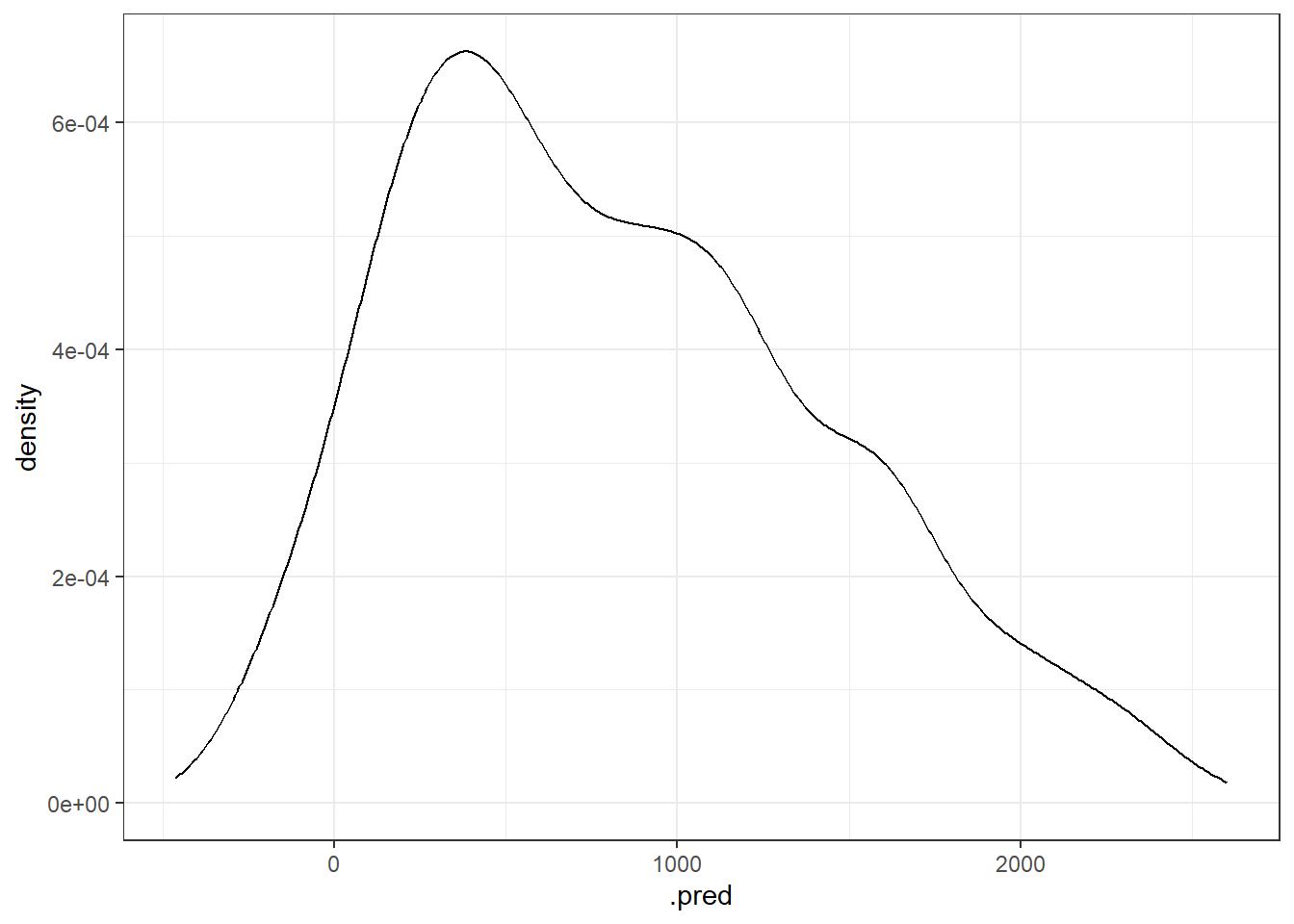
## 1 rmse standard 351.ggplot(test_preds, aes(x=.pred)) +
geom_density()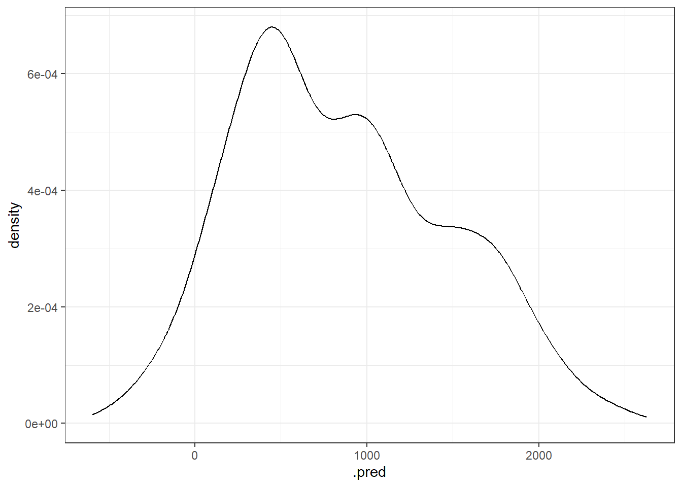
divvy_data <- divvy_data %>%
  mutate(
    day = floor_date(started_hour, 'day'),
    bad_weather = if_else(solar_rad <= 5 & temp <= 5, 1, 0),
    nice_weather = if_else(solar_rad >= 25 & temp >= 15, 1, 0)
  )

total_rain <- divvy_data %>% group_by(
  day
) %>% summarize(total_precip = sum(interval_rain, na.rm=T))

divvy_data <- divvy_data %>% left_join(total_rain) %>%
  mutate(rainy_weather = if_else(total_precip > 0, 1, 0))

grouped <- rsample::initial_split(divvy_data)
train <- training(grouped)
test  <- testing(grouped)

lm_model <-
  parsnip::linear_reg() %>%
  set_engine("lm") %>%
  fit(rides ~ solar_rad + factor(hour(started_hour)) +
        factor(nice_weather) + factor(bad_weather) + factor(rainy_weather) +
        temp + avg_speed, data=train)

preds <-
  predict(lm_model, test %>% filter(month(started_hour) >= 5))

test_preds <- lm_model %>%
  augment(test %>% filter(month(started_hour) >=5))

yardstick::mape(test_preds,
     truth = rides,
     estimate = .pred)
## # A tibble: 1 × 3
## .metric .estimator .estimate
## <chr> <chr> <dbl>
## 1 mape standard 97.0yardstick::rmse(test_preds,
truth = rides,
estimate = .pred)## # A tibble: 1 × 3
## .metric .estimator .estimate
## <chr> <chr> <dbl>
## 1 rmse standard 357.ggplot(test_preds, aes(x=.pred)) +
geom_density()