Make a classification model and run evaluations.
Part A
We are going to use a toy dataset called bivariate. There is a training, testing, and validation dataset provided.
library(tidyverse)
## Warning: package 'tidyverse' was built under R version 4.1.3
## -- Attaching packages --------------------------------------- tidyverse 1.3.2 --
## v ggplot2 3.4.0      v purrr   0.3.5
## v tibble  3.1.8      v dplyr   1.0.10
## v tidyr   1.2.1      v stringr 1.5.0
## v readr   2.1.3      v forcats 0.5.2
## Warning: package 'ggplot2' was built under R version 4.1.3
## Warning: package 'tibble' was built under R version 4.1.3
## Warning: package 'tidyr' was built under R version 4.1.3
## Warning: package 'readr' was built under R version 4.1.3
## Warning: package 'purrr' was built under R version 4.1.3
## Warning: package 'dplyr' was built under R version 4.1.3
## Warning: package 'stringr' was built under R version 4.1.3
## Warning: package 'forcats' was built under R version 4.1.3
## -- Conflicts ------------------------------------------ tidyverse_conflicts() --
## x dplyr::filter() masks stats::filter()
## x dplyr::lag()    masks stats::lag()
library(tidymodels)
## Warning: package 'tidymodels' was built under R version 4.1.3
## -- Attaching packages -------------------------------------- tidymodels 1.0.0 --
## v broom        1.0.1     v rsample      1.1.1
## v dials        1.1.0     v tune         1.0.1
## v infer        1.0.4     v workflows    1.1.2
## v modeldata    1.0.1     v workflowsets 1.0.0
## v parsnip      1.0.3     v yardstick    1.1.0
## v recipes      1.0.3
## Warning: package 'broom' was built under R version 4.1.3
## Warning: package 'dials' was built under R version 4.1.3
## Warning: package 'scales' was built under R version 4.1.3
## Warning: package 'infer' was built under R version 4.1.3
## Warning: package 'modeldata' was built under R version 4.1.3
## Warning: package 'parsnip' was built under R version 4.1.3
## Warning: package 'recipes' was built under R version 4.1.3
## Warning: package 'rsample' was built under R version 4.1.3
## Warning: package 'tune' was built under R version 4.1.3
## Warning: package 'workflows' was built under R version 4.1.3
## Warning: package 'workflowsets' was built under R version 4.1.3
## Warning: package 'yardstick' was built under R version 4.1.3
## -- Conflicts ----------------------------------------- tidymodels_conflicts() --
## x scales::discard() masks purrr::discard()
## x dplyr::filter()   masks stats::filter()
## x recipes::fixed()  masks stringr::fixed()
## x dplyr::lag()      masks stats::lag()
## x yardstick::spec() masks readr::spec()
## x recipes::step()   masks stats::step()
## * Use suppressPackageStartupMessages() to eliminate package startup messages
theme_set(theme_bw())

data(bivariate)

ggplot(bivariate_train, aes(x=A, y=B, color=Class)) +
  geom_point(alpha=.3)
Use logistic_reg and glm to make a classification model of Class ~ A * B. Then use tidy and glance to see some summary information on our model. Anything stand out to you?
log_model <- logistic_reg() %>%
  set_engine('glm') %>%
  set_mode('classification') %>%
  fit(Class ~ A*B,
      data = bivariate_train)

log_model %>% tidy()
## # A tibble: 4 x 5
##   term          estimate  std.error statistic  p.value
##   <chr>            <dbl>      <dbl>     <dbl>    <dbl>
## 1 (Intercept)  0.115     0.404          0.284 7.76e- 1
## 2 A            0.00433   0.000434       9.97  2.01e-23
## 3 B           -0.0553    0.00633       -8.74  2.32e-18
## 4 A:B         -0.0000101 0.00000222    -4.56  5.04e- 6
log_model %>% broom::glance()
## # A tibble: 1 x 8
##   null.deviance df.null logLik   AIC   BIC deviance df.residual  nobs
##           <dbl>   <int>  <dbl> <dbl> <dbl>    <dbl>       <int> <int>
## 1         1329.    1008  -549. 1106. 1126.    1098.        1005  1009
Part B
Use augment to get predictions. Look at the predictions.
test_preds <- log_model %>% augment(bivariate_test)

test_preds
## # A tibble: 710 x 6
##        A     B Class .pred_class .pred_One .pred_Two
##    <dbl> <dbl> <fct> <fct>           <dbl>     <dbl>
##  1  742.  68.8 One   One           0.730      0.270
##  2  709.  50.4 Two   Two           0.491      0.509
##  3 1006.  89.9 One   One           0.805      0.195
##  4 1983. 112.  Two   Two           0.431      0.569
##  5 1698.  81.0 Two   Two           0.169      0.831
##  6  948.  98.9 One   One           0.900      0.0996
##  7  751.  54.8 One   One           0.521      0.479
##  8 1254.  72.2 Two   Two           0.347      0.653
##  9 4243. 136.  One   Two           0.00568    0.994
## 10  713.  88.2 One   One           0.910      0.0898
## # ... with 700 more rows
Part C
Visually inspect the predictions using the code below
# log_model, your parnsip model
# bivariate_train / bivariate_val, data from bivariate

# to plot the countour we need to create a grid of points and get the model prediction at each point
x_grid <-
  expand.grid(A = seq(min(bivariate_train$A), max(bivariate_train$A), length.out = 100),
              B = seq(min(bivariate_train$B), max(bivariate_train$B), length.out = 100))
x_grid_preds <- log_model %>% augment(x_grid)

# plot predictions from grid as countour and validation data on plot
ggplot(x_grid_preds, aes(x = A, y = B)) +
  geom_contour(aes(z = .pred_One), breaks = .5, col = "black") +
  geom_point(data = bivariate_val, aes(col = Class), alpha = 0.3)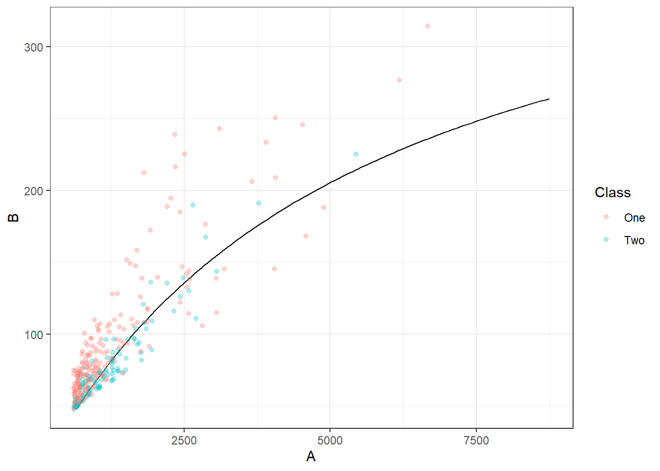
Part D
Evaluate your model using the following functions (which dataset(s) should you use to do this train, test, or validation). See if you can provide a basic interpretation of the measures.
- roc_auc
- accuracy
- roc_curve and autoplot
- f_meas
val_preds <- log_model %>% augment(bivariate_val)

val_preds %>% roc_auc(truth = Class,
                      estimate = .pred_One)
## # A tibble: 1 x 3
##   .metric .estimator .estimate
##   <chr>   <chr>          <dbl>
## 1 roc_auc binary         0.790

val_preds %>% accuracy(truth = Class,
                      estimate = .pred_class)
## # A tibble: 1 x 3
##   .metric  .estimator .estimate
##   <chr>    <chr>          <dbl>
## 1 accuracy binary          0.76


roc_curve(val_preds,
        truth = Class,
        estimate = .pred_One) %>%
  autoplot()
f_meas(val_preds,
        truth = Class,
        estimate = .pred_class)
## # A tibble: 1 x 3
##   .metric .estimator .estimate
##   <chr>   <chr>          <dbl>
## 1 f_meas  binary         0.827
Part E
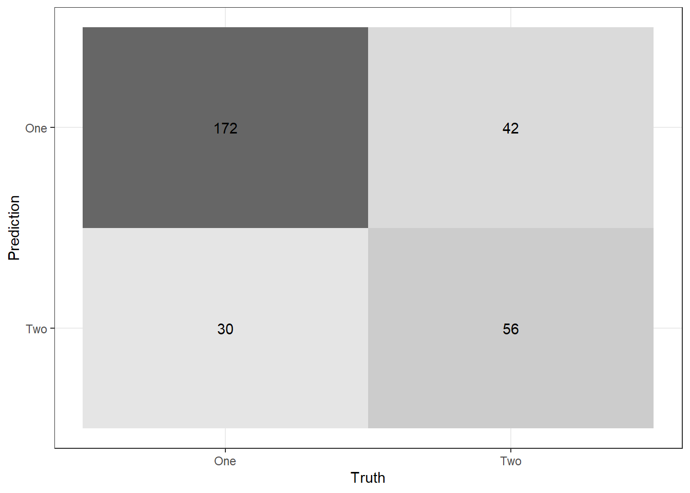
Recall Table 8.4 from the textbook. If necessary, class one can be positive and class two can be negative. Using the output from conf_mat, visually verify you know how to calculate the following:
- True Positive Rate (TPR), Sensitivity, or Recall
- True Negative Rate (TNR) or Specificity
- False Positive Rate, Type I error
- False Negative Rate (FNR), Type II error
- Positive Predictive Value (PPV) or Precision
val_preds %>% conf_mat(truth = Class,
                      estimate = .pred_class) %>%
  autoplot("heatmap")